Category: Research
Learning Skills to Navigate without a Master: A Sequential Multi-Policy Reinforcement Learning Algorithm
General Information
- Learning Skills to Navigate without a Master: A Sequential Multi-Policy Reinforcement Learning Algorithm
- Ambedkar Dukkipati, Rajarshi Banerjee, Ranga Shaarad Ayyagari, Dhaval Parmar Udaybhai
- Indian Institute of Science
- A. Dukkipati, R. Banerjee, R. S. Ayyagari and D. P. Udaybhai, "Learning Skills to Navigate without a Master: A Sequential Multi-Policy Reinforcement Learning Algorithm," 2022 IEEE/RSJ International Conference on Intelligent Robots and Systems (IROS), Kyoto, Japan, 2022, pp. 2483-2489, doi: 10.1109/IROS47612.2022.9981607.
Learning Skills to Navigate without a Master: A Sequential Multi-Policy Reinforcement Learning Algorithm
Abstract
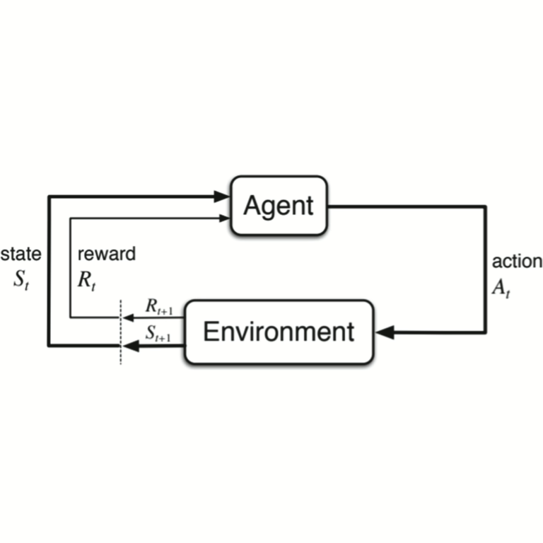
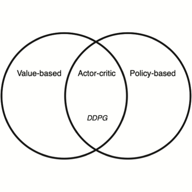
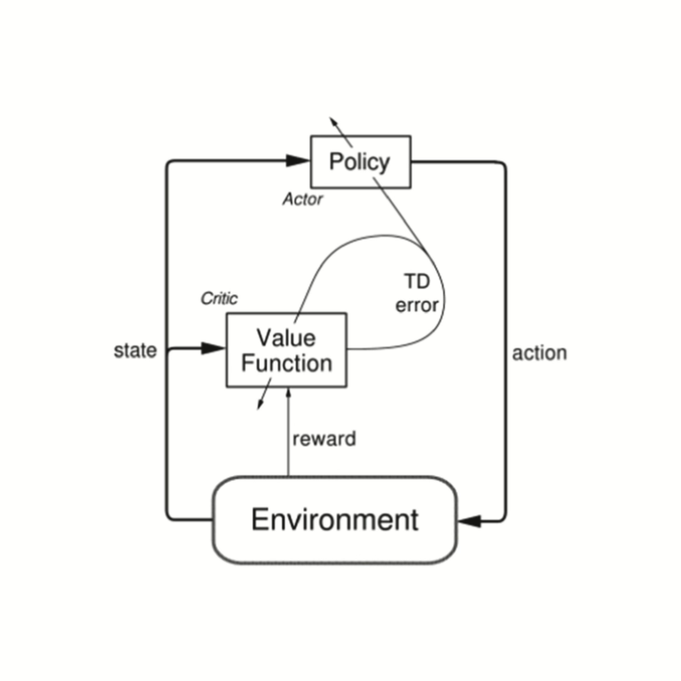
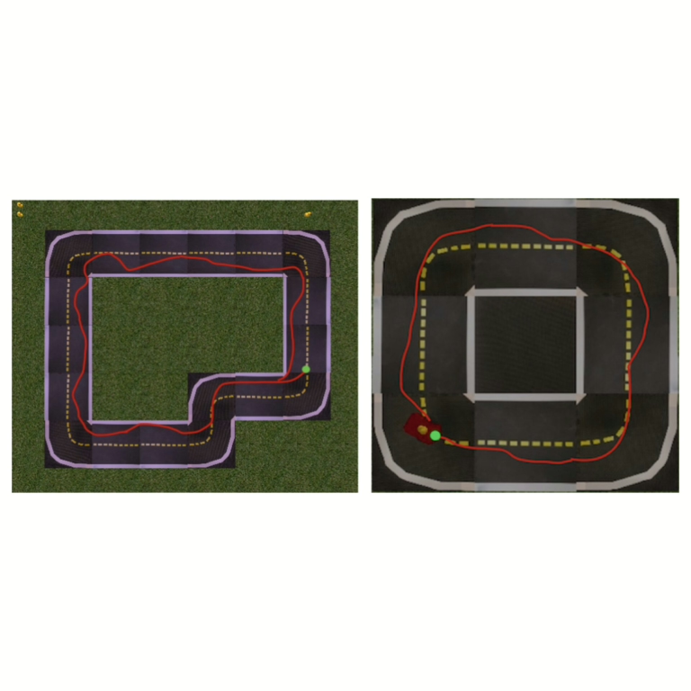
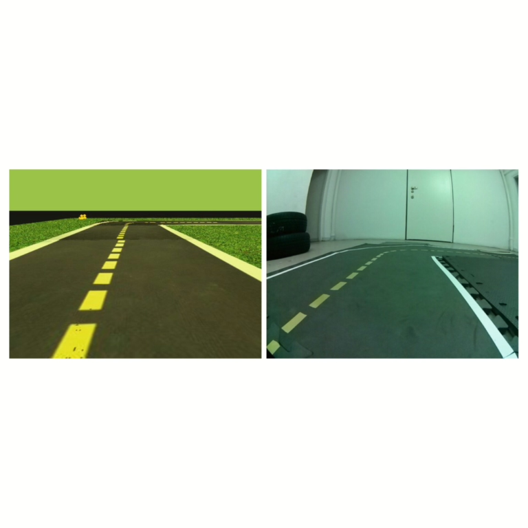
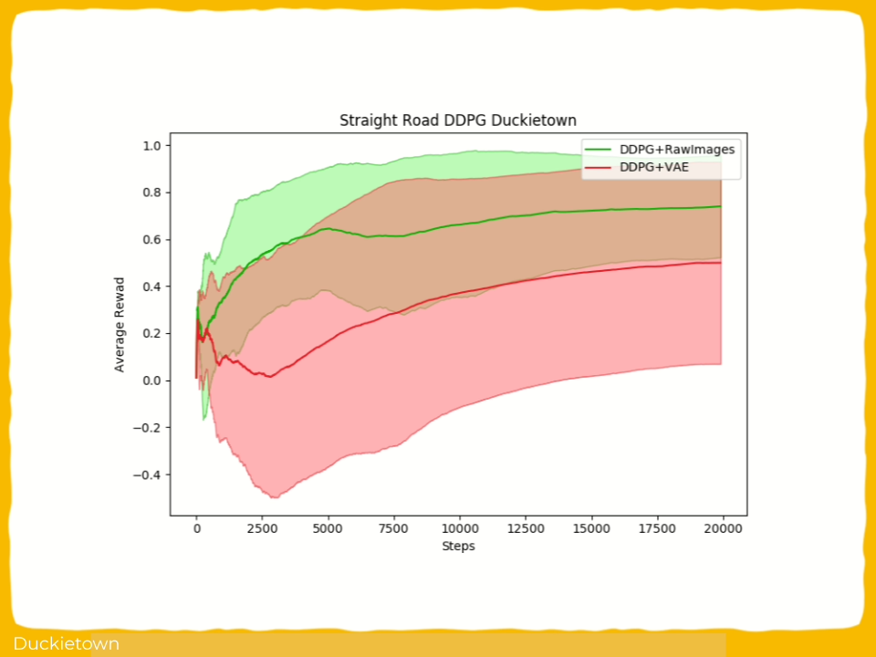
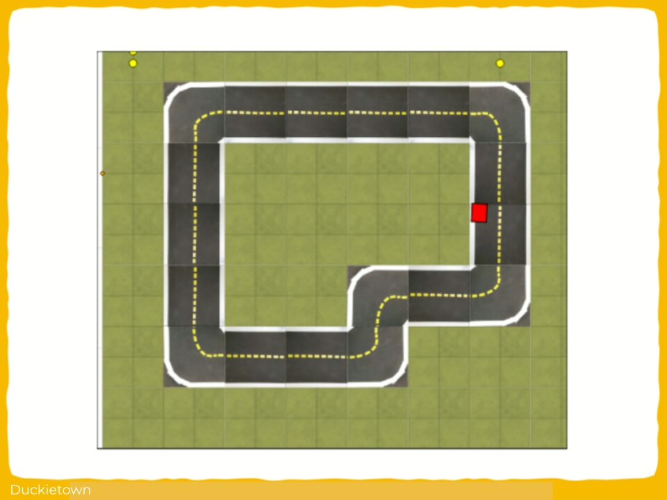
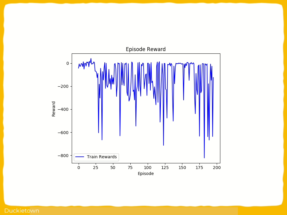
Solving complex problems using reinforcement learning necessitates breaking down the problem into manageable tasks, and learning policies to solve these tasks. These policies, in turn, have to be controlled by a master policy that takes high-level decisions. Hence learning policies involves hierarchical decision structures. However, training such methods in practice may lead to poor generalization, with either sub-policies executing actions for too few time steps or devolving into a single policy altogether. In our work, we introduce an alternative approach to learn such skills sequentially without using an overarching hierarchical policy. We propose this method in the context of environments where a major component of the objective of a learning agent is to prolong the episode for as long as possible. We refer to our proposed method as Sequential Soft Option Critic. We demonstrate the utility of our approach on navigation and goal-based tasks in a flexible simulated 3D navigation environment that we have developed. We also show that our method outperforms prior methods such as Soft Actor-Critic and Soft Option Critic on various environments, including the Atari River Raid environment and the Gym-Duckietown self-driving car simulator.
Highlights
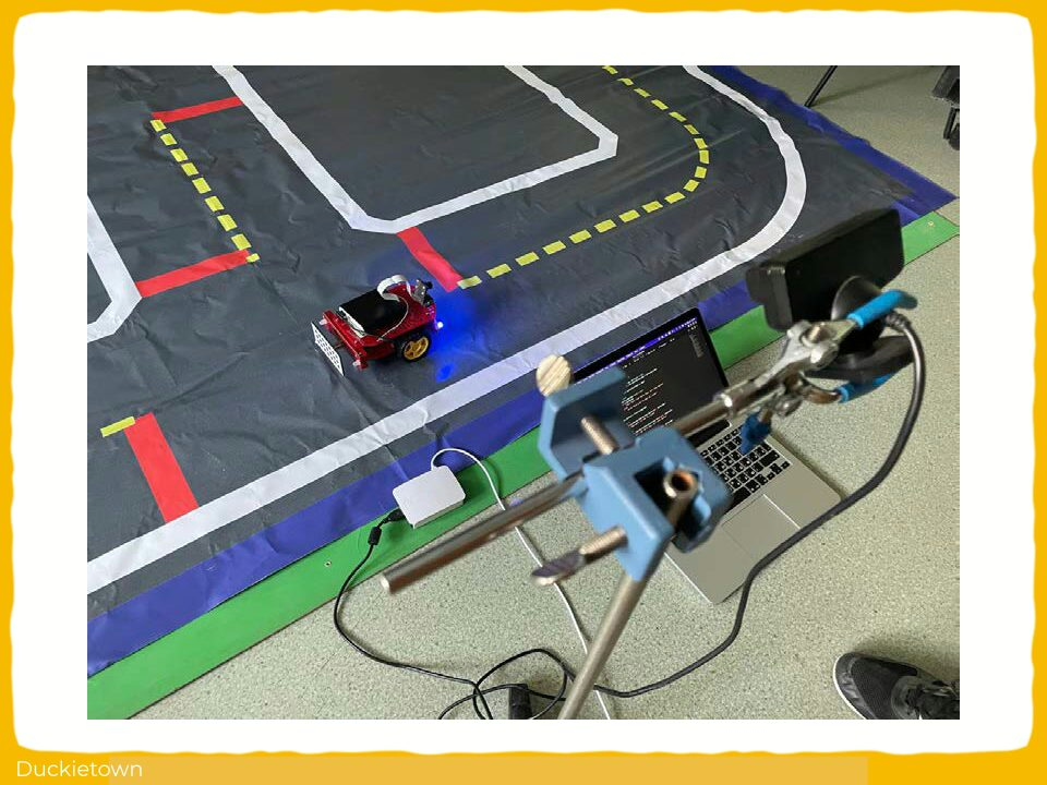
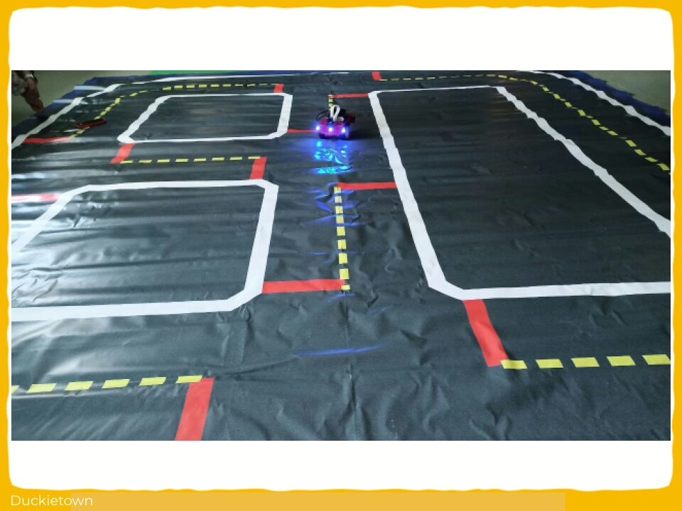
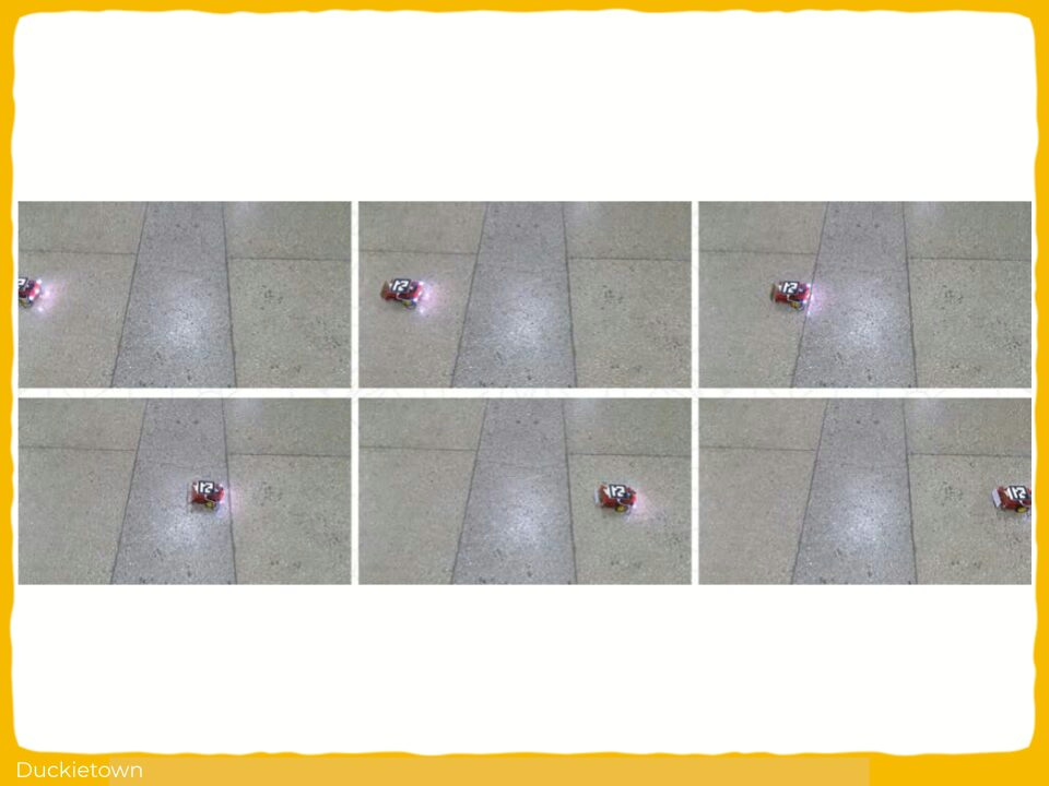
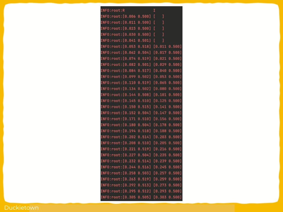
Here is a visual tour of the work of the authors.
For all the details, check out the paper link!
Conclusion
Learn more
Duckietown is a platform for creating and disseminating robotics and AI learning experiences.
Duckietown is modular, customizable and state-of-the-art. It is designed to teach, learn, and do research: from exploring the fundamentals of computer science and automation to pushing the boundaries of knowledge.
Monocular Robot Navigation with Self-Supervised Pretrained Vision Transformers
Monocular Robot Navigation with Self-Supervised Pre-trained Vision Transformers
Duckietown’s infrastructure is used by researchers worldwide to push the boundaries of knowledge. Of the many outstanding works published, today we’d like to highlight “Monocular Robot Navigation with Self-Supervised Pretrained Vision Transformers” by Saavedra-Ruiz et al. at the University of Montreal.
Using visual transformers (ViT) for understanding their surroundings, Duckiebots are made capable of detecting and avoiding obstacles, while safely driving inside lanes. ViT is an emerging machine vision technique that has its root in Natural Language Processing (NLP) applications. The use of this architecture is recent and promising in Computer Vision. Enjoy the read and don’t forget to reproduce these results on your Duckiebots!
Abstract
“In this work, we consider the problem of learning a perception model for monocular robot navigation using few annotated images. Using a Vision Transformer (ViT) pretrained with a label-free self-supervised method, we successfully train a coarse image segmentation model for the Duckietown environment using 70 training images. Our model performs coarse image segmentation at the 8×8 patch level, and the inference resolution can be adjusted to balance prediction granularity and real-time perception constraints. We study how best to adapt a ViT to our task and environment, and find that some lightweight architectures can yield good single-image segmentations at a usable frame rate, even on CPU. The resulting perception model is used as the backbone for a simple yet robust visual servoing agent, which we deploy on a differential drive mobile robot to perform two tasks: lane following and obstacle avoidance.”
Pipeline
“We propose to train a classifier to predict labels for every 8×8 patch in an image. Our classifier is a fully-connected network which we apply over ViT patch encodings to predict a coarse segmentation mask:”
Conclusions
Learn more
The Duckietown platform offers robotics and AI learning experiences.
Duckietown is modular, customizable and state-of-the-art. It is designed to teach, learn, and do research: from exploring the fundamentals of computer science and automation to pushing the boundaries of knowledge.
AI Driving Olympics 2021: Urban League Finalists
AI Driving Olympics 2021 - Urban League Finalists
LF
), lane following with vehicles (LFV
) and lane following with intersections, (LFI
).
To account for differences between the real world and simulation, this edition finalists can make one additional submission to the real
challenges to improve their scores.
Finalists are the authors of AI-DO 2021 submissions in the top 5 ranks for each challenge.
This year’s finalists are: LF
- András Kalapos
- Bence Haromi
- Sampsa Ranta
- ETU-JBR Team
- Giulio Vaccari
LFV
- Sampsa Ranta
- Adrian Brucker
- Andras Beres
- David Bardos
LFI
- András Kalapos
- Sampsa Ranta
- Adrian Brucker
- Andras Beres
The deadline for submitting the “final” submissions is Dec. 9th, 2 pm CET. All submissions received after this time will count towards the next edition of AI-DO.
Don’t forget to join the #aido channel on the Duckietown Slack for updates!
Congratulations to all the participants, and best of luck to the finalists!
Join the AI Driving Olympics, 6th edition, starting now!
The 2021 AI Driving Olympics
Compete in the 2021 edition of the Artificial Intelligence Driving Olympics (AI-DO 6)!
The AI-DO serves to benchmark the state of the art of artificial intelligence in autonomous driving by providing standardized simulation and hardware environments for tasks related to multi-sensory perception and embodied AI.
Duckietown traditionally hosts AI-DO competitions biannually, with finals events held at machine learning and robotics conferences such as the International Conference on Robotics and Automation (ICRA) and the Neural Information Processing Systems (NeurIPS).
AI-DO 6 will be in conjunction with NeurIPS 2021 and have three leagues: urban driving, advanced perception, and racing. The winter champions will be announced during NeurIPS 2021, on December 10, 2021!
Urban driving league
The urban driving league uses the Duckietown platform and presents several challenges, each of increasing complexity.
The goal in each challenge is to develop a robotic agent for driving Duckiebots “well”. Baseline implementations are provided to test different approaches. There are no constraints on how your agents are designed.
Each challenge adds a layer of complexity: intersections, other vehicles, pedestrians, etc. You can check out the existing challenges on the Duckietown challenges server.
AI-DO 2021 features four challenges: lane following (LF
), lane following with intersections (LFI
), lane following with vehicles (LFV
) and lane following with vehicles and intersections, multi-body, with full information (LFVI-multi-full
).
All challenges have a simulation and hardware component (,), except for LFVI-multi-full
, which is simulation () only.
The first phase (until Nov. 7) is a practice one. Results do not count towards leaderboards.
The second phase (Nov. 8-30) is the live competition and results count towards official leaderboards.
Selected submissions (that perform well enough in simulation) will be evaluated on hardware in Autolabs. The submissions scoring best in Autolabs will access the finals.
During the finals (Dec. 1-8) one additional submission is possible for each finalist, per challenge.
Winners (top 3) of the resulting leaderboard will be declared AI-DO 2021 winter champions and celebrated live during NeurIPS 2021. We require champions to submit a short video (2 mins) introducing themselves and describing their submission.
Winners are invited to join (not mandatory) the NeurIPS event, on December 10th, 2021, starting at 11.25 GMT (Zoom link will follow).
Overview
🎯 | Goal: develop robotic agents for challenges of increasing complexity |
🚙 | Robot: Duckiebot (DB21M/J ) |
👀 | Sensors: camera, wheel encoders |
Schedule
Practice: Nov. 1-7 | |
Competition: Nov. 8-30 | |
Finals: Dec. 1 – 8 | |
Winners: Dec. 10 |
Rules
Practice: unlimited non-competing submissions | |
Competition: best in sim are evaluated on hardware in Autolabs | |
Finals: one additional submission for Autolabs | |
Winners: 2 mins video submission description for NeurIPS 2021 event. |
The challenges
Lane following
LF
– The most traditional of AI-DO challenges: have a Duckiebot navigate a road loop without intersection, pedestrians (duckies) nor other vehicles. The objective is to travel the longest path in a given time while staying in the lane, i.e., not committing driving infractions.
Current AI-DO leaderboards: LF-sim-validation, LF-sim-testing.
Previous AI-DO leaderboards: sim-validation, sim-testing, real-validation.
Lane following with intersections
LFI
– This challenge builds upon LF
by increasing the complexity of the road network, now featuring 3 and/or 4-way intersections, defined according to the Duckietown appearance specifications. Traffic lights will not be present on the map. The objective is to drive the longest distance while not breaking the rules of the road, now more complex due to the presence of traffic signs.
Current AI-DO leaderboards: LFI-sim-validation, LFI-sim-testing.
Previous AI-DO leaderboards: sim-validation, sim-testing.
Lane following with vehicles
LFV
– In this traditional AI-DO challenge, contestants seek to travel the longest path in a city without intersections nor pedestrians, but with other vehicles on the road. Non-playing vehicles (i.e., not running the user’s submitted agent) can be in the same and/or opposite lanes and have variable speed. Current AI-DO leaderboards: LFV-sim-validation, LFV-sim-testing.
Lane following with vehicles and intersections (stateful)
LFVI-multi-full
– this debuting challenge brings together roads with intersections and other vehicles. The submitted agent is deployed on all Duckiebots on the map (-multi
), and is provided with full information, i.e., the state of the other vehicles on the map (-full
). This challenge is in simulation only. Leaderboards: LFVI_multi_full-sim-validation
Getting started
All you need to get started and participate in the AI-DO is a computer, a good internet connection, and the ambition to challenge your skills against the international community!
We provide webinars, operation manuals, and baselines to get started.
May the duck be with you!
Thank you to our generous sponsors!
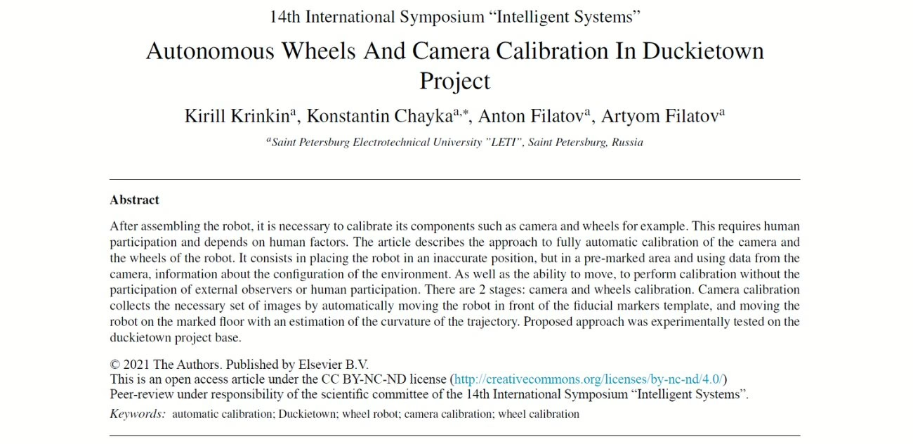
Automatic Wheels and Camera Calibration for Monocular and Differential Mobile Robots
- Automatic Wheels and Camera Calibration for Monocular and Differential Mobile Robots
- Konstantin Chaika, Anton Filatov, Artyom Filatov, Kirill Krinkin
- Applied Sciences 11, no. 13: 5806.
Automatic Wheels and Camera Calibration for Monocular and Differential Mobile Robots
After assembling the robot, components such as the camera and wheels need to be calibrated. This requires human participation and depends on human factors. We describe the approach to fully automatic calibration of a robot’s camera and wheels.
The camera calibration collects the necessary set of images by automatically moving the robot in front of the chess boards, and then moving it on the marked floor, assessing its trajectory curvature. As a result of the calibration, coefficient k is calculated for the wheels, and camera matrix K (which includes the focal length, the optical center, and the skew coefficient) and distortion coefficients D are calculated for the camera.
Proposed approach has been tested on duckiebots in Alexander Popov’s International Innovation Institute for Artificial Intelligence, Cybersecurity and Communication, SPbETU “LETI”. This solution is comparable to manual calibrations and is capable of replacing a human for this task.
Camera calibration process
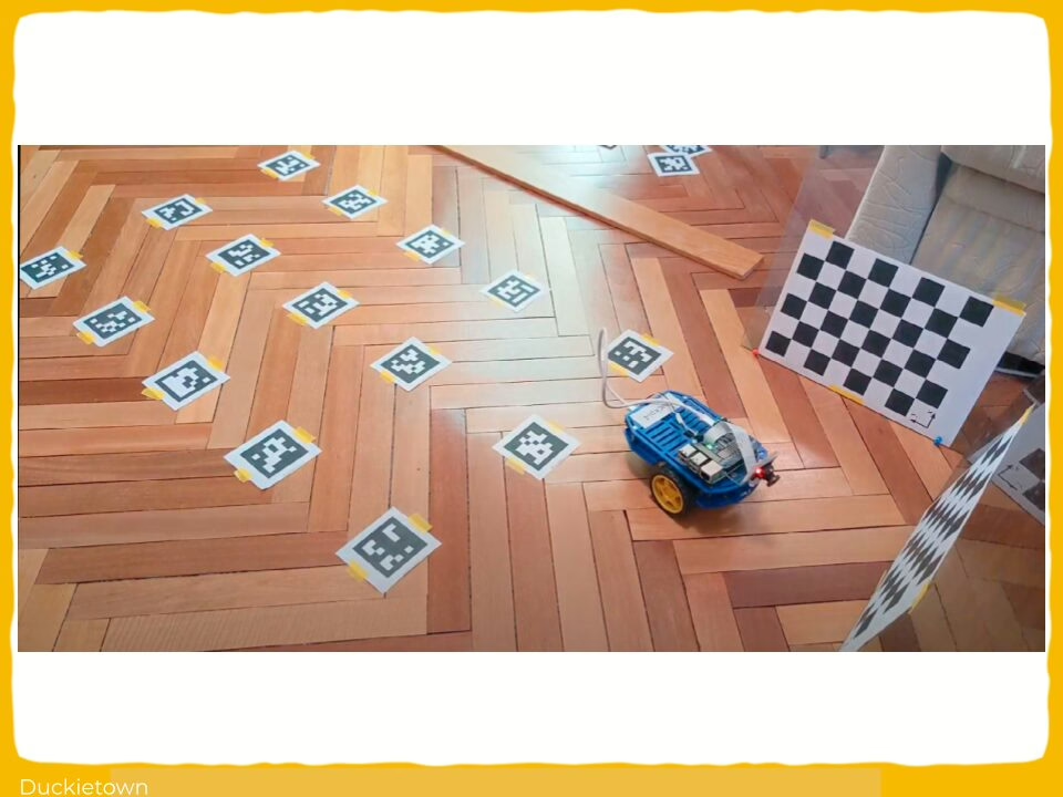
The initial position of the robot is a part of the floor with chessboards in front, where the robot is located from the very beginning, on which its camera is directed and the floorsurface is marked with aruco markers on the other side of it.
There can be any number of chessboards, determined by the amount of free space around the robot. To a greater extent, the accuracy of calibration is affected by the frames with different positions of the boards, e.g., boards located at different distances from the robot and at different angles. The physical size and type of all the boards around the robot must be the same.
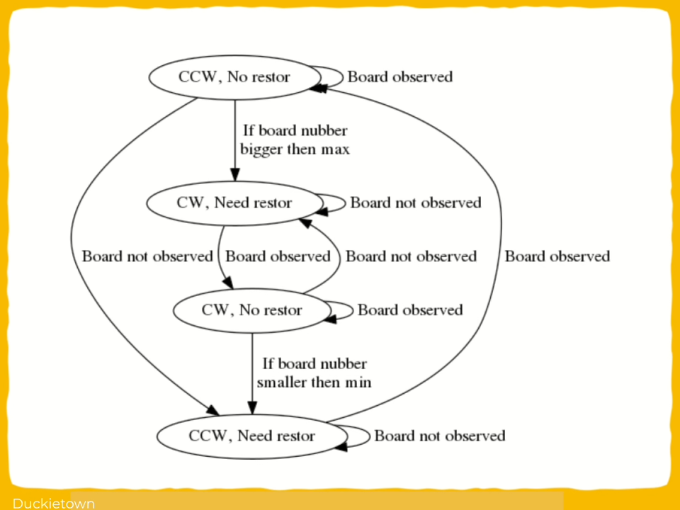
In fact, the camera calibration implies that the robot is rotating around its axis and taking pictures of all the viewable chessboards in turn. In this case, the ability to make several “passes” during the shooting process should be provided for, to control which of the boards the robot is currently observing and in which direction it should turn. As a result, the algorithm can be represented as a sequence of actions: “get a frame from the camera” and “turn” a little. The final algorithm comprises the following sequence of actions:
- Obtain frame from the camera;
- Find a chessboard on the camera frame;
- Save information about board corners found in the image;
- Determine the direction of rotation according to the schedule;
- Make a step;
- Either repeat the steps described above, or complete the data
collection and proceed with the camera calibration using OpenCV.
Wheels calibration process
Floor markers should be oriented towards the chessboards and begin as close to the robot as possible. The distance between the markers depends on camera’s resolution, as well as its height and angle of inclination, but it must be such that at least three recognizable markers can simultaneously be in the frame. For ours experiments, the distance between the markers was set as 15 cm with a marker size of 6.5 cm. The algorithm does not take into account the relative position of the markers against each other; however, the orientation of all markers must be strictly the same.
Let us consider the first iteration of the automatic wheel calibration algorithm:
- The robot receives the orientation of the marker closest to it and remembers it.
- Next, the robot moves forward with thespeeds of the left and right wheels equal to
ω1ω2 for some fixed time t. The speeds are calculated taking into account the calibration
coefficient k, which for the first iteration is chosen to equal 1 – that is, it is assumed that
the real wheel speeds are equal. - The robot obtains the orientation of the marker closest to it again and calculates the
difference in angles between them. - The coefficient ki for this step is calculated.
- The robot moves back for the same time t.
In order to reduce the influence of the error in calculating ki, coefficient k is refined only by the value of (ki−1)/2 after each iteration. It is important to complete this step after the robot moves back, because it reduces the chance of the robot moving outside the area width. If, after the next step, the modulus of the difference between (ki−1)/2 and 1.0 becomes less than the pre-selected E, then at this iteration (ki−1)/2 is not taken into account. If after three successive iterations ki is not taken into account, the wheel calibration is considered to be completed.
Accuracy Evaluation
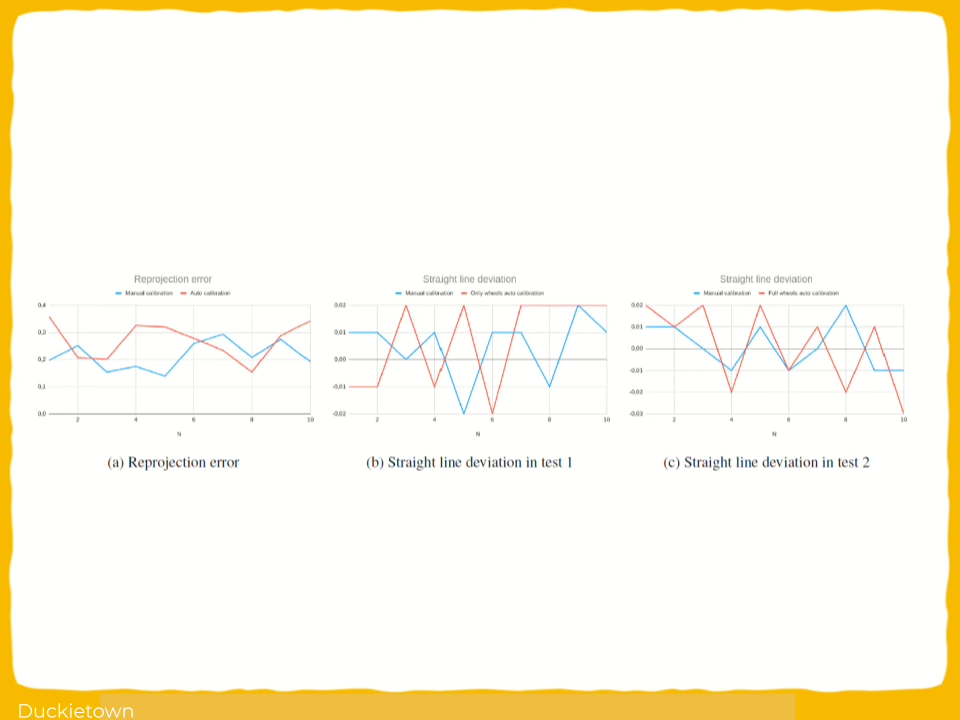
To compare camera calibration errors, the knowledge of how to calculate these errors is needed. Since the calibration mechanism is used by the OpenCV library, the error is also calculated by the method offered by this library.
As noted earlier, with respect to calibration factors, the approach used to calibrate the camera is not applicable. Therefore, the influence of the coefficient on the robot’s trajectory curvature is estimated. To do this, the robot was located at a certain fixed distance from a straight line, along which it was oriented and then moved in manual mode strictly directly to a distance of two meters from the start point along the axis, relative to which it was oriented. Then, the robot stopped and the distance between the initial distance to the line and the final one was calculated.
Two metrices were estimated – reprojection error and straight line deviation. First one shows the quality of camera calibration, and the second one represents the quality of wheels calibration. Two pictures below present result of 10 independent tests in comparison with manual calibration.
The tests found that the suggested solution, on average, shows that the results are not much worse, than the classical manual solution when calibrating the camera, as well as when calibrating the wheels with a well known calibrated camera. However, when calibrating both the wheels and the camera, the wheel calibration can be significantly affected by the camera calibration effect. As a result of testing, a clear relationship was found between the reprojection error and the straight line deviation.
Method Modifications
After the integration of this approach, it became necessary to automate the last step-moving the robot to the field. Due to the fact that after the calibration step completion the robot becomes fully prepared for launching autonomous driving algorithms on it, the automation of this step further reduces the time spent by the operator when calibrating the robot, since instead of moving the robot to the field manually, he can place the next robot at the starting position. In our case, the calibration field was located at the side of the road lane so that the floor markers used to calibrate the wheels are oriented perpendicular to the road lane.
Thus, the first stage of the robot automatic removal from the calibration zone is to return its orientation back to the same state, as it was at the moment when the wheel calibration started. This was carried out using exactly the same approach that was described earlier—depending on the orientation of the floor marker closest to the robot, the robot rotates step by step about its axis clockwise or counterclockwise until the value of the robot’s orientation angle is modulo less than some preselected value.
At this point, the robot is still on the wheel calibration field, but in this case, it is oriented towards the lane. Thus, the last step is to move the robot outside the border of the field with markers. To do this, it is enough to give the robot a command to move directly until it stops observing the markers, when the last marker is hidden from the camera view. This means that the robot has left the calibration zone, and the robot can be put into the lane following mode.
Future Work
During the robot’s operation, the wheels calibration may become irrelevant. It can be influenced by various factors: a change in the wheel diameter due to wear of the wheel coating, a slight change in the characteristics of motors due to the wear of the gearbox plastic, and a change in the robot’s weight distribution, e.g., laying the cables on the other side of the case after charging the robot, and so a slight calibration mismatch can occur. However, all these factors have a rather small impact, and the robot will still have a satisfactory calibration. There is no need to re-perform the calibration process, just a little refinement of the current one seems to be enough. To do this, a section of the road along which the robots will be guaranteed to pass regularly, was selected.
Further, markers were placed in this lane according to the rules described earlier: the distance between the markers is 15 cm; the size of the marker is 6.5 cm. The markers are located in the center of the lane. The distance between the markers may be not completely accurate, but they should be oriented in the same direction and co-directed with the movement in the lane on which they are placed.
The first marker in the direction of travel must have a predefined ID. It can be anything, the only limitation is that it must be unique for a current robot environment. Further, the following changes were made to the algorithm for the standard control of the robot: when the robot recognizes the first marker with a predetermined ID while driving right in the lane, it corrects its orientation relative to this marker and continues to move strictly straight ahead. Further, the algorithm is similar to the one described earlier—the robot recognizing the next marker can refine its wheel calibration coefficient, apply it, and change the orientation coaxially with the next marker.
Conclusions
As a result, a solution was developed that allows a fully automatic calibration of the camera and the Duckiebot’s wheels. The main feature is the autonomy of the process, which allows one person to run the calibration of an arbitrary number of robots in parallel and not be blocked during their calibration. In addition, the robot is able to improve its calibration as it operates in default mode.
Comparing the developed solution with the initial one resulted in finding a slight deterioration in accuracy, which is primarily associated with the accuracy of the camera calibration; however, the result obtained is sufficient for the robot’s initial calibration and is comparable to manual calibration.
Did you find this interesting?
Read more Duckietown based papers here.
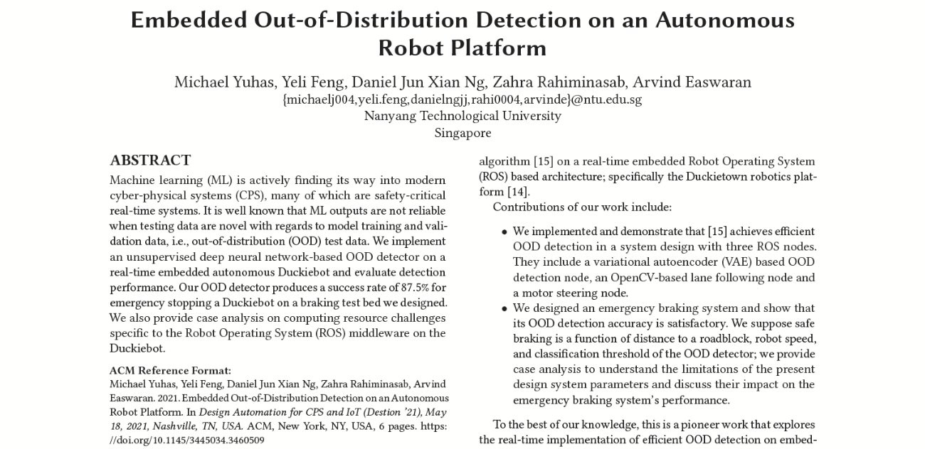
Embedded out-of-distribution detection on an autonomous robot platform
- Embedded out-of-distribution detection on an autonomous robot platform
- Michael Yuhas, Yeli Feng, Daniel Jun Xian Ng, Zahra Rahiminasab, Arvind Easwa M ran
- Design Automation for CPS and IoT (DESTION 2021) Workshop
- ACM Digital Library
- Code available here
- Data available here
Introduction
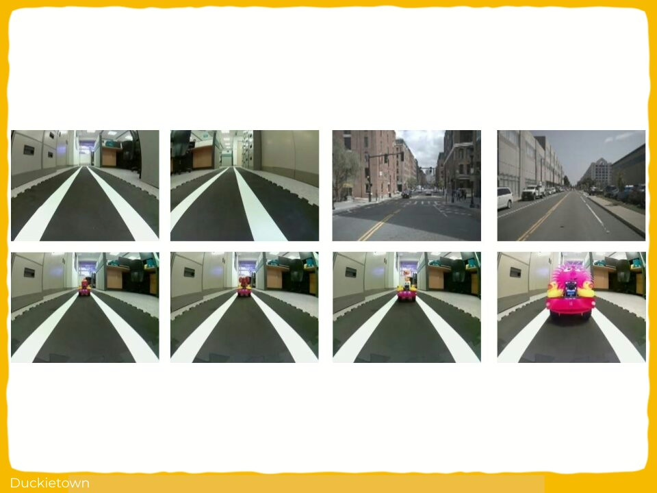
Machine learning is becoming more and more common in cyber-physical systems; many of these systems are safety critical, e.g. autonomous vehicles, UAVs, and surgical robots. However, machine learning systems can only provide accurate outputs when their input data is similar to their training data. For example, if an object detector in an autonomous vehicle is trained on images containing various classes of objects, but no ducks, what will it do when it encounters a duck during runtime? One method for dealing with this challenge is to detect inputs that lie outside the training distribution of data: out-of-distribution (OOD) detection. Many OOD detector architectures have been explored, however the cyber-physical domain adds additional challenges: hard runtime requirements and resource constrained systems. In this paper, we implement a real-time OOD detector on the Duckietown framework and use it to demonstrate the challenges as well as the importance of OOD detection in cyber-physical systems.
Out-of-Distribution Detection
Machine learning systems perform best when their test data is similar to their training data. In some applications unreliable results from a machine learning algorithm may be a mere nuisance, but in other scenarios they can be safety critical. OOD detection is one method to ensure that machine learning systems remain safe during test time. The goal of the OOD detector is to determine if the input sample is from a different distribution than that of the training data. If an OOD sample is detected, the detector can raise a flag indicating that the output of the machine learning system should not be considered safe, and that the system should enter a new control regime. In an autonomous vehicle, this may mean handing control back to the driver, or bringing the vehicle to a stop as soon as practically possible.
In this paper we consider the existing β-VAE based OOD detection architecture. This architecture takes advantage of the information bottleneck in a variational auto-encoder (VAE) to learn the distribution of training data. In this detector the VAE undergoes unsupervised training with the goal of minimizing the error between a true prior probability in input space p(z), and an approximated posterior probability from the encoder output p(z|x). During test time, the Kullback-Leibler divergence between these distributions p(z) and q(z|x) will be used to assign an OOD score to each input sample. Because the training goal was to minimize the distance between these two distributions on in-distribution data, in-distribution data found at runtime should have a low OOD score while OOD data should have a higher OOD score.
Duckietown
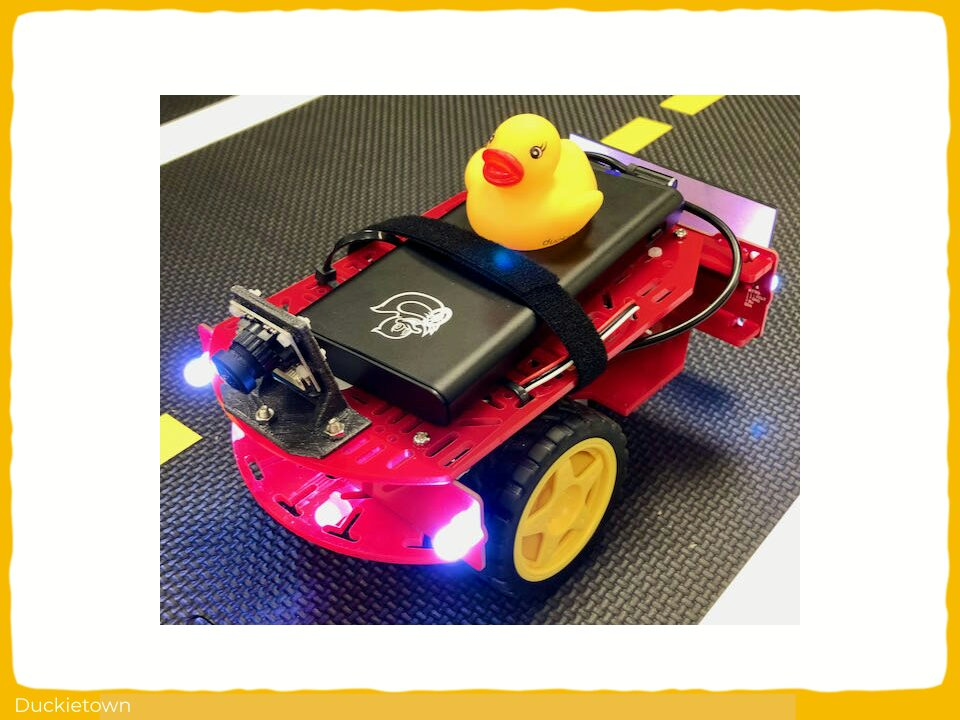
We used Duckietown to implement our OOD detector. Duckietown provides a natural test bed because:
- It is modular and easy to learn: the focus of our research is about implementing an OOD detector, not building a robot from scratch
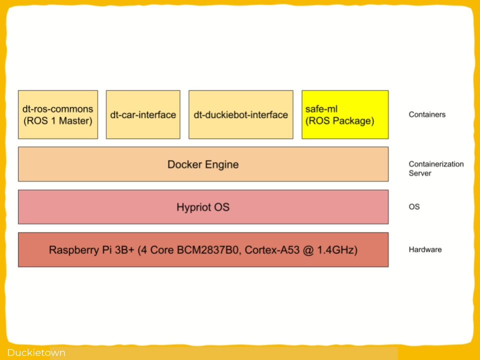
- It is a resource constrained system: the RPi on the DB18 is powerful enough to be capable of navigation tasks, but resource constrained enough that real-time performance is not guaranteed. It servers as a good analog for a system in which an OOD detector shares a CPU with perception, planning, and control software.
- It is open source: this eliminates the need to purchase and manage licenses, allows us to directly check the source code when we encounter implementation issues, and allows us to contribute back to the community once our project is finished.
- It is low-cost: we’re not made of money 🙂
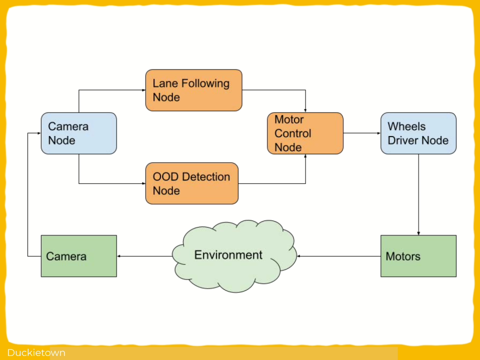
- Lane following node: a simple OpenCV-based lane follower that navigates based on camera images. This represents the perception and planning system for the mobile robot that we are trying to protect. In our system the lane following node takes 640×480 RGB images and updates the planned trajectory at a rate of 5Hz.
- OOD detection node: this node also takes images directly from the camera, but its job is to raise a flag when an OOD input appears (image with an OOD score greater than some threshold). On the RPi with no GPU or TPU, it takes a considerable amount of time to make an inference on the VAE, so our detection node does not have a target rate, but rather uses the last available camera frame, dropping any frames that arrive while the OOD score is being computed.
- Motor control node: during normal operation it takes the trajectory planned by the lane following node and sends it to the wheels. However, if it receives a signal from the OOD detection node, it begins emergency breaking.
The Experiment
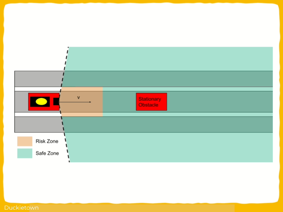
Our experiment considers the emergency stopping distance required for the Duckiebot when an OOD input is detected. In our setup the Duckiebot drives forward along a straight track. The area in front of the robot is divided into two zones: the risk zone and the safe zone. The risk zone is an area where if an obstacle appears, it poses a risk to the Duckiebot. The safe zone is further away and to the sides; this is a region where unknown obstacles may be present, but they do not pose an immediate threat to the robot. An obstacle that has not appeared in the training set is placed in the safe zone in front of the robot. As the robot drives forward along the track, the obstacle will eventually enter the risk zone. Upon entry into the risk zone we measure how far the Duckiebot travels before the OOD detector triggers an emergency stop.
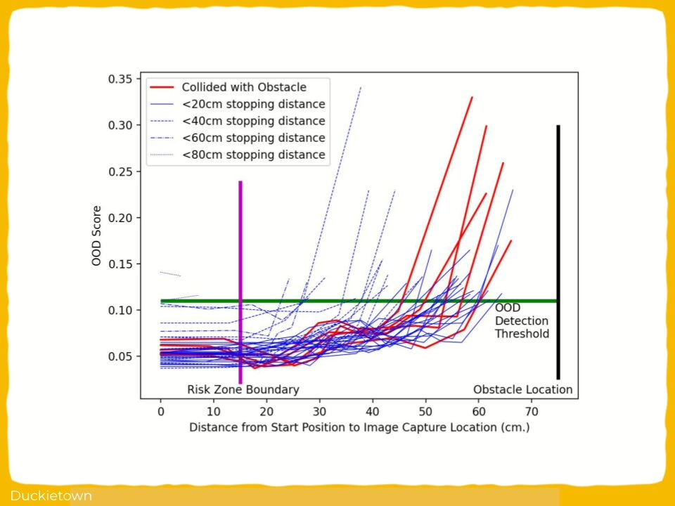
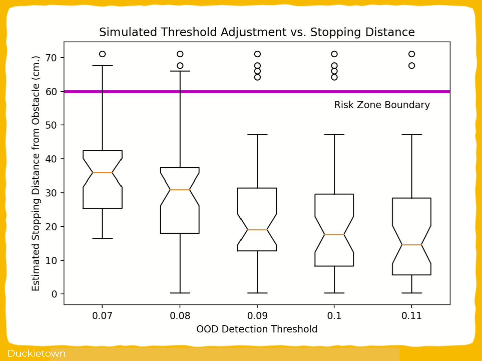
We defined the risk zone as the area 60cm directly in front of our Duckiebot. We repeated the experiment 40 times and found that with our system architecture, the Duckiebot stopped on average 14.5cm before the obstacle. However, in 5 iterations of the experiment, the Duckiebot collided with the stationary obstacle.
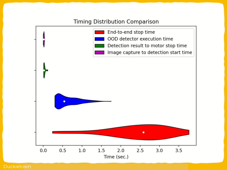
We wanted to analyze what lead to the collision in those five cases. We started by looking at the times it took for our various nodes to run. We plotted the distribution of end-to-end stopping times, image capture to detection start times, OOD detector execution times, and detection result to motor stop times. We observed that there was a long tail on the OOD execution times, which lead us to suspect that the collisions occurred when the OOD detector took too long to produce a result. This hypothesis was bolstered by the fact that even when a collision had occurred, the last logged OOD score was above the detection threshold, it had just been produced too late. We also looked at the final two OOD detection times for each collision and found that in every case the final two times were above the median detector execution time. This highlights the importance of real-time scheduling when performing OOD detection in a cyber-physical system.
We also wanted to analyze what would happen if we adjusted the OOD detection threshold. Because we had logged the the detection threshold every time the detector had run, we were able to interpolate the position of the robot at every detection time and discover when the robot would have stopped for different OOD detection thresholds. We observe there is a tradeoff associated with moving the detection threshold. If the detection threshold is lowered, the frequency of collisions can be reduced and even eliminated. However, the mean stopping distance is also moved further from the obstacle and the robot is more likely to stop spuriously when the obstacle is outside of the risk zone.
Next Steps
In this paper we successfully implemented an OOD detector on a mobile robot, but our experiment leaves many more questions:
- How does the performance of other OOD detector architectures compare with the β-VAE detector we used in this paper?
- How can we guarantee the real-time performance of an OOD detector on a resource-constrained system, especially when sharing a CPU with other computationally intensive tasks like perception, planning, and control?
- Does the performance vary when detecting more complex OOD scenarios: dynamic obstacles, turning corners, etc.?
Did you find this interesting?
Read more Duckietown based papers here.
AI Driving Olympics 5th edition: results
AI-DO 5: Urban league winners
This year’s challenges were lane following (LF
), lane following with pedestrians (LFP
) and lane following with other vehicles, multibody (LFV_multi
).
Let’s find out the results in each category:
LF
- Andras Beres 🇭🇺
- Zoltan Lorincz 🇭🇺
- András Kalapos 🇭🇺
LFP
- Bea Baselines 🐤
- Melisande Teng 🇨🇦
- Raphael Jean 🇨🇦
LFV_multi
- Robert Moni 🇭🇺
- Márton Tim 🇭🇺
- Anastasiya Nikolskay 🇷🇺
Congratulations to the Hungarian Team from the Budapest University of Technology and Economics for collecting the highest rankings in the urban league!
Here’s how the winners in each category performed both in the qualification (simulation) and in the finals running on real hardware:
Andras Beres - Lane following (LF) winner
Melisande Teng - Lane following with pedestrians (LFP) winner
Robert Moni - Lane following with other vehicles, multibody (LFV_multi) winner
AI-DO 5: Advanced Perception league winners
Great participation and results in the Advanced Perception league! Check out this year’s winners in the video below:
AI-DO 5 sponsors
Many thanks to our amazing sponsors, without which none of this would have been possible!
Stay tuned for next year AI Driving Olympics. Visit the AI-DO page for more information on the competition and to browse this year’s introductory webinars, or check out the Duckietown massive open online course (MOOC) and prepare for next year’s competition!
AI-DO 5 competition leaderboard update
AI-DO 5 pre-finals update
With the fifth edition of the AI Driving Olympics finals day approaching, 1326 solutions submitted from 94 competitors in three challenges, it is time to glance over at the leaderboards!
Leaderboards updates
LF
), lane following with pedestrians (LFP
) and lane following with other vehicles, multibody (LFV_multi
). Learn more about the challenges here.
Each submission can be sent to multiple challenges.
Let’s look at some of the most promising or interesting submissions. The Montréal menace
Raphael Jean at Mila / University of Montréal is a new entrant for this year.
An interesting submission: submission #12962
The submissions from the cold
Team JetBrains from Saint Petersburg was a winner of previous editions of AI-DO. They have been dominating the leaderboards also this year.
Interesting submissions: submission #12905
All of JetBrains submissions: JBRRussia1.
BME Conti
PhD student Robert Moni (BME-Conti) from Hungary.
Interesting submissions: submission #12999
All submissions: timur-BMEconti
Deadline for submissions
Imitation Learning Approach for AI Driving Olympics Trained on Real-world and Simulation Data Simultaneously
- Imitation Learning Approach for AI Driving Olympics Trained on Real-world and Simulation Data Simultaneously
- Mikita Sazanovich, Konstantin Chaika, Kirill Krinkin, Aleksei Shpilman
- Workshop on AI for Autonomous Driving (AIAD), the 37th International Conference on Machine Learning, Vienna, Austria, 2020
- ArXiv version download: arXiv:2007.03514
- Find code here
Imitation Learning Approach for AI Driving Olympics Trained on Real-world and Simulation Data Simultaneously
The AIDO challenge is divided into two global stages: simulation and real-world. A single algorithm needs to perform well in both. It was quickly identified that one of the major problems is the simulation to real-world transfer.
Many algorithms trained in the simulated environment performed very poorly in the real world, and many classic control algorithms that are known to perform well in a real-world environment, once tuned to that environment, do not perform well in the simulation. Some approaches suggest randomizing the domain for the simulation to real-world transfer.
We propose a novel method of training a neural network model that can perform well in diverse environments, such as simulations and real-world environment.
Dataset Generation
To that end, we have trained our model through imitation learning on a dataset compiled from four different sources:
- Real-world Duckietown dataset from logs.duckietown.com (REAL-DT).
- Simulation dataset on a simple loop map (SIM-LP).
- Simulation dataset on an intersection map (SIM-IS).
- Real-world dataset collected by us in our environment with car driven by PD controller (REAL-IH).
We aimed to collect data with as many possible situations such as twists in the road, driving in circles clockwise/counterclockwise, and so on. We have also tried to diversify external factors such as scene lighting, items in the room that can get into the camera’s field of view, roadside objects, etc. If we keep these conditions constant, our model may overfit to them and perform poorly in a different environment. For this reason, we changed the lighting and environment after each duckiebot run. The lane detection was calibrated for every lighting condition since different lighting changes the color scheme of the image input.
We made the following change to the standard PD algorithm: since most Duckietown turns and intersections are standard-shaped, we hard-coded the robot’s motion in these situations, but we did not exclude imperfect trajectories. For example, the ones that would go slightly out of bounds of the lane. Imperfections in the robot’s actions increase the robustness of the model.
Neural network architecture and training
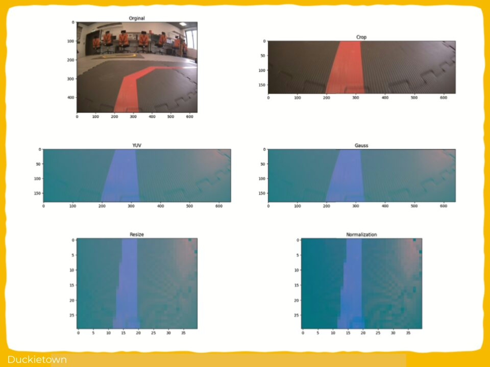
Original images are 640×480 RGB. As a preprocessing step, we remove the top third of the image, since it mostly contains the sky, resize the image to 64×32 pixels and convert it into the YUV colorspace.
We have used 5 convolutional layers with a small number of filters, followed by 2 fully-connected layers. The small size of the network is not only due to it being less prone to overfitting, but we also need a model that can run on a single CPU on RaspberryPi.
We have also incorporated Independent-Component (IC) layers. These layers aim to make the activations of each layer more independent by combining two popular techniques, BatchNorm and Dropout. For convolutional layers, we substitute Dropout with Spatial Dropout which has been shown to work better with them. The model outputs two values for voltages of the left and the right wheel drives. We use the mean square error (MSE) as our training loss.
Results
For the training evaluation, we compute the mean square error (MSE) of the left and the right wheels outputs on the validation set of each data source.
The first table shows the results for the models trained on all data sources (HYBRID), on real-world data sources only (REAL) and on simulation data sources only (SIM). As we can see, while training on a single dataset sometimes achieves lower error on the same dataset than our hybrid approach. We can also see that our method performs on par with the best single methods. In terms of the average error it outperforms the closest one tenfold. This demonstrates definitively the high dependence of MSE on the training method, and highlights the differences between the data sources.
The next table shows simulation closed-loop performance for all our approaches using the Duckietown simulator. All methods drove for 15 seconds without major infractions, and the SIM model that was trained specifically on the simulation data only drove just 1.8 tiles more than our hybrid approach.
The third table shows the closed-loop performance in the real-world environment. Comparing the number of tiles, we see that our hybrid approach drove about 3.5 tiles more than the following in the rankings model trained on real-world data only.
Conclusion
Our method follows the imitation learning approach and consists of a convolutional neural network which is trained on a dataset compiled from data from different sources, such as simulation model and real-world Duckietown vehicle driven by a PD controller, tuned to various conditions, such as different map configuration and lighting.
We believe that our approach of emphasizing neurons independence and monitoring generalization performance can offer more robustness to control models that have to perform in diverse environments. We also believe that the described approach of imitation learning on data obtained from several algorithms that are fitted to specific environments may yield a single algorithm that will perform well in general.