Konstantin Chaika - Duckietown

Automatic Wheels and Camera Calibration for Monocular and Differential Mobile Robots

After assembling the robot, components such as the camera and wheels need to be calibrated. This requires human participation and depends on human factors. We describe the approach to fully automatic calibration of a robot’s camera and wheels.

The camera calibration collects the necessary set of images by automatically moving the robot in front of the chess boards, and then moving it on the marked floor, assessing its trajectory curvature. As a result of the calibration, coefficient k is calculated for the wheels, and camera matrix K (which includes the focal length, the optical center, and the skew coefficient) and distortion coefficients D are calculated for the camera.

Proposed approach has been tested on duckiebots in Alexander Popov’s International Innovation Institute for Artificial Intelligence, Cybersecurity and Communication, SPbETU “LETI”. This solution is comparable to manual calibrations and is capable of replacing a human for this task.

Camera calibration process

The initial position of the robot is a part of the floor with chessboards in front, where the robot is located from the very beginning, on which its camera is directed and the floorsurface is marked with aruco markers on the other side of it.

There can be any number of chessboards, determined by the amount of free space around the robot. To a greater extent, the accuracy of calibration is affected by the frames with different positions of the boards, e.g., boards located at different distances from the robot and at different angles. The physical size and type of all the boards around the robot must be the same.

In fact, the camera calibration implies that the robot is rotating around its axis and taking pictures of all the viewable chessboards in turn. In this case, the ability to make several “passes” during the shooting process should be provided for, to control which of the boards the robot is currently observing and in which direction it should turn. As a result, the algorithm can be represented as a sequence of actions: “get a frame from the camera” and “turn” a little. The final algorithm comprises the following sequence of actions:

Obtain frame from the camera;
Find a chessboard on the camera frame;
Save information about board corners found in the image;
Determine the direction of rotation according to the schedule;
Make a step;
Either repeat the steps described above, or complete the data
collection and proceed with the camera calibration using OpenCV.

Wheels calibration process

Floor markers should be oriented towards the chessboards and begin as close to the robot as possible. The distance between the markers depends on camera’s resolution, as well as its height and angle of inclination, but it must be such that at least three recognizable markers can simultaneously be in the frame. For ours experiments, the distance between the markers was set as 15 cm with a marker size of 6.5 cm. The algorithm does not take into account the relative position of the markers against each other; however, the orientation of all markers must be strictly the same.

Let us consider the first iteration of the automatic wheel calibration algorithm:

The robot receives the orientation of the marker closest to it and remembers it.
Next, the robot moves forward with thespeeds of the left and right wheels equal to
ω₁ω₂ for some fixed time t. The speeds are calculated taking into account the calibration
coefficient k, which for the first iteration is chosen to equal 1 – that is, it is assumed that
the real wheel speeds are equal.
The robot obtains the orientation of the marker closest to it again and calculates the
difference in angles between them.
The coefficient k_i for this step is calculated.
The robot moves back for the same time t.

In order to reduce the influence of the error in calculating ki, coefficient k is refined only by the value of (k_i−1)/2 after each iteration. It is important to complete this step after the robot moves back, because it reduces the chance of the robot moving outside the area width. If, after the next step, the modulus of the difference between (k_i−1)/2 and 1.0 becomes less than the pre-selected E, then at this iteration (k_i−1)/2 is not taken into account. If after three successive iterations k_i is not taken into account, the wheel calibration is considered to be completed.

Accuracy Evaluation

To compare camera calibration errors, the knowledge of how to calculate these errors is needed. Since the calibration mechanism is used by the OpenCV library, the error is also calculated by the method offered by this library.

As noted earlier, with respect to calibration factors, the approach used to calibrate the camera is not applicable. Therefore, the influence of the coefficient on the robot’s trajectory curvature is estimated. To do this, the robot was located at a certain fixed distance from a straight line, along which it was oriented and then moved in manual mode strictly directly to a distance of two meters from the start point along the axis, relative to which it was oriented. Then, the robot stopped and the distance between the initial distance to the line and the final one was calculated.

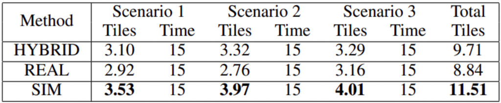
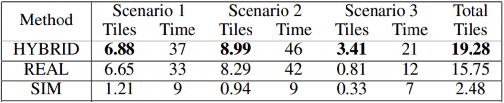
Two metrices were estimated – reprojection error and straight line deviation. First one shows the quality of camera calibration, and the second one represents the quality of wheels calibration. Two pictures below present result of 10 independent tests in comparison with manual calibration.

The tests found that the suggested solution, on average, shows that the results are not much worse, than the classical manual solution when calibrating the camera, as well as when calibrating the wheels with a well known calibrated camera. However, when calibrating both the wheels and the camera, the wheel calibration can be significantly affected by the camera calibration effect. As a result of testing, a clear relationship was found between the reprojection error and the straight line deviation.

Method Modifications

After the integration of this approach, it became necessary to automate the last step-moving the robot to the field. Due to the fact that after the calibration step completion the robot becomes fully prepared for launching autonomous driving algorithms on it, the automation of this step further reduces the time spent by the operator when calibrating the robot, since instead of moving the robot to the field manually, he can place the next robot at the starting position. In our case, the calibration field was located at the side of the road lane so that the floor markers used to calibrate the wheels are oriented perpendicular to the road lane.

Thus, the first stage of the robot automatic removal from the calibration zone is to return its orientation back to the same state, as it was at the moment when the wheel calibration started. This was carried out using exactly the same approach that was described earlier—depending on the orientation of the floor marker closest to the robot, the robot rotates step by step about its axis clockwise or counterclockwise until the value of the robot’s orientation angle is modulo less than some preselected value.

At this point, the robot is still on the wheel calibration field, but in this case, it is oriented towards the lane. Thus, the last step is to move the robot outside the border of the field with markers. To do this, it is enough to give the robot a command to move directly until it stops observing the markers, when the last marker is hidden from the camera view. This means that the robot has left the calibration zone, and the robot can be put into the lane following mode.

Future Work

During the robot’s operation, the wheels calibration may become irrelevant. It can be influenced by various factors: a change in the wheel diameter due to wear of the wheel coating, a slight change in the characteristics of motors due to the wear of the gearbox plastic, and a change in the robot’s weight distribution, e.g., laying the cables on the other side of the case after charging the robot, and so a slight calibration mismatch can occur. However, all these factors have a rather small impact, and the robot will still have a satisfactory calibration. There is no need to re-perform the calibration process, just a little refinement of the current one seems to be enough. To do this, a section of the road along which the robots will be guaranteed to pass regularly, was selected.

Further, markers were placed in this lane according to the rules described earlier: the distance between the markers is 15 cm; the size of the marker is 6.5 cm. The markers are located in the center of the lane. The distance between the markers may be not completely accurate, but they should be oriented in the same direction and co-directed with the movement in the lane on which they are placed.

The first marker in the direction of travel must have a predefined ID. It can be anything, the only limitation is that it must be unique for a current robot environment. Further, the following changes were made to the algorithm for the standard control of the robot: when the robot recognizes the first marker with a predetermined ID while driving right in the lane, it corrects its orientation relative to this marker and continues to move strictly straight ahead. Further, the algorithm is similar to the one described earlier—the robot recognizing the next marker can refine its wheel calibration coefficient, apply it, and change the orientation coaxially with the next marker.

Conclusions

As a result, a solution was developed that allows a fully automatic calibration of the camera and the Duckiebot’s wheels. The main feature is the autonomy of the process, which allows one person to run the calibration of an arbitrary number of robots in parallel and not be blocked during their calibration. In addition, the robot is able to improve its calibration as it operates in default mode.

Comparing the developed solution with the initial one resulted in finding a slight deterioration in accuracy, which is primarily associated with the accuracy of the camera calibration; however, the result obtained is sufficient for the robot’s initial calibration and is comparable to manual calibration.

Did you find this interesting?

Imitation Learning Approach for AI Driving Olympics Trained on Real-world and Simulation Data Simultaneously

The AIDO challenge is divided into two global stages: simulation and real-world. A single algorithm needs to perform well in both. It was quickly identified that one of the major problems is the simulation to real-world transfer.

Many algorithms trained in the simulated environment performed very poorly in the real world, and many classic control algorithms that are known to perform well in a real-world environment, once tuned to that environment, do not perform well in the simulation. Some approaches suggest randomizing the domain for the simulation to real-world transfer.

We propose a novel method of training a neural network model that can perform well in diverse environments, such as simulations and real-world environment.

Dataset Generation

To that end, we have trained our model through imitation learning on a dataset compiled from four different sources:

Real-world Duckietown dataset from logs.duckietown.com (REAL-DT).
Simulation dataset on a simple loop map (SIM-LP).
Simulation dataset on an intersection map (SIM-IS).
Real-world dataset collected by us in our environment with car driven by PD controller (REAL-IH).

We aimed to collect data with as many possible situations such as twists in the road, driving in circles clockwise/counterclockwise, and so on. We have also tried to diversify external factors such as scene lighting, items in the room that can get into the camera’s field of view, roadside objects, etc. If we keep these conditions constant, our model may overfit to them and perform poorly in a different environment. For this reason, we changed the lighting and environment after each duckiebot run. The lane detection was calibrated for every lighting condition since different lighting changes the color scheme of the image input.

We made the following change to the standard PD algorithm: since most Duckietown turns and intersections are standard-shaped, we hard-coded the robot’s motion in these situations, but we did not exclude imperfect trajectories. For example, the ones that would go slightly out of bounds of the lane. Imperfections in the robot’s actions increase the robustness of the model.

Neural network architecture and training

Original images are 640×480 RGB. As a preprocessing step, we remove the top third of the image, since it mostly contains the sky, resize the image to 64×32 pixels and convert it into the YUV colorspace.

We have used 5 convolutional layers with a small number of filters, followed by 2 fully-connected layers. The small size of the network is not only due to it being less prone to overfitting, but we also need a model that can run on a single CPU on RaspberryPi.

We have also incorporated Independent-Component (IC) layers. These layers aim to make the activations of each layer more independent by combining two popular techniques, BatchNorm and Dropout. For convolutional layers, we substitute Dropout with Spatial Dropout which has been shown to work better with them. The model outputs two values for voltages of the left and the right wheel drives. We use the mean square error (MSE) as our training loss.

Results

For the training evaluation, we compute the mean square error (MSE) of the left and the right wheels outputs on the validation set of each data source.

The first table shows the results for the models trained on all data sources (HYBRID), on real-world data sources only (REAL) and on simulation data sources only (SIM). As we can see, while training on a single dataset sometimes achieves lower error on the same dataset than our hybrid approach. We can also see that our method performs on par with the best single methods. In terms of the average error it outperforms the closest one tenfold. This demonstrates definitively the high dependence of MSE on the training method, and highlights the differences between the data sources.

The next table shows simulation closed-loop performance for all our approaches using the Duckietown simulator. All methods drove for 15 seconds without major infractions, and the SIM model that was trained specifically on the simulation data only drove just 1.8 tiles more than our hybrid approach.

The third table shows the closed-loop performance in the real-world environment. Comparing the number of tiles, we see that our hybrid approach drove about 3.5 tiles more than the following in the rankings model trained on real-world data only.

Conclusion

Our method follows the imitation learning approach and consists of a convolutional neural network which is trained on a dataset compiled from data from different sources, such as simulation model and real-world Duckietown vehicle driven by a PD controller, tuned to various conditions, such as different map configuration and lighting.

We believe that our approach of emphasizing neurons independence and monitoring generalization performance can offer more robustness to control models that have to perform in diverse environments. We also believe that the described approach of imitation learning on data obtained from several algorithms that are fitted to specific environments may yield a single algorithm that will perform well in general.

—

JBRRussia1 team