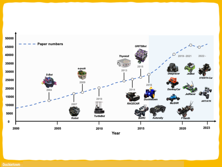
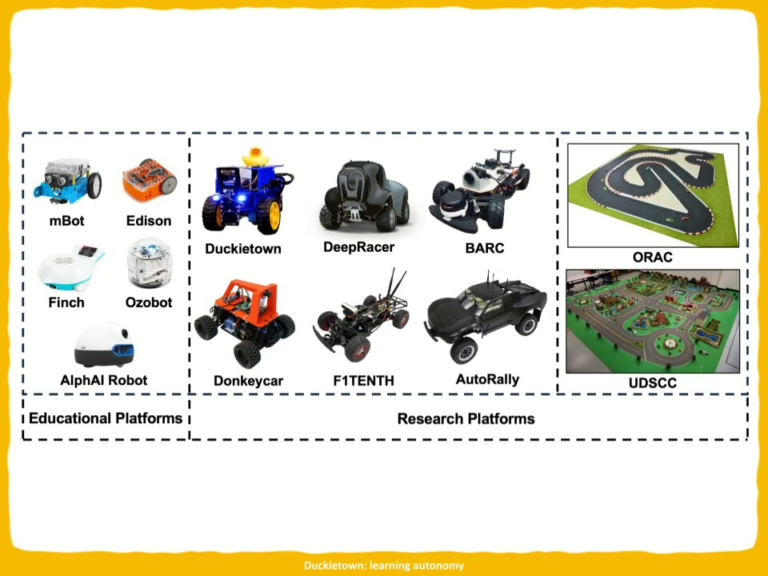
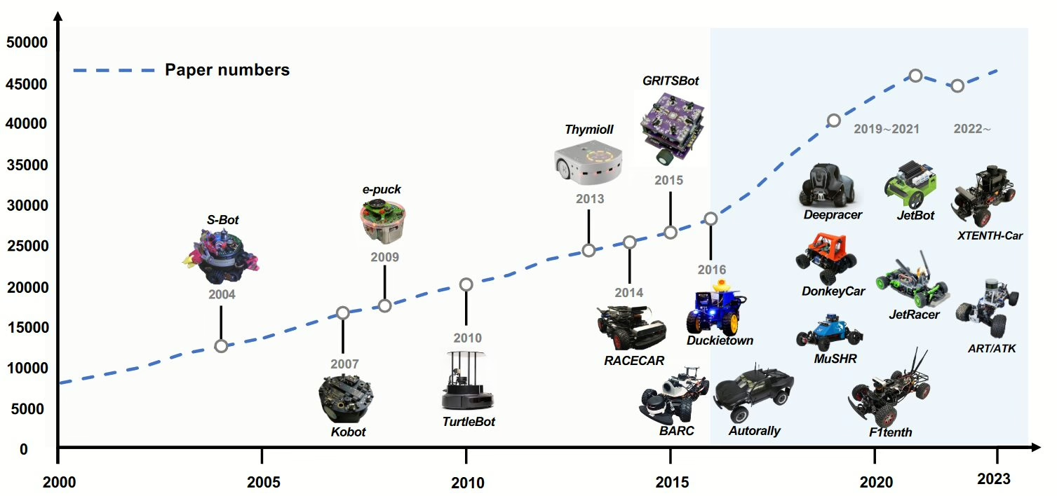
“Towards Autonomous Driving with Small-Scale Cars: A Survey of Recent Development by Dianzhao Li, Paul Auerbach, and Ostap Okhrin is a review that highlights the rapid development of the industry and the important contributions of small-scale car platforms to robot autonomy research.
This survey is a valuable resource for anyone looking to get their bearings in the landscape of autonomous driving research.
We are glad see Duckietown – not only included on the list – but identified as one of the platforms that started a marked increase in the trend of yearly published papers.
The mission of Duckietown, since we started at as a class at MIT, is to democratize access to the science and technology of robot autonomy. Part of how we intended to achieve this mission was to streamline the way autonomous behaviors for non-trivial robots were developed, tested and deployed in the real world.
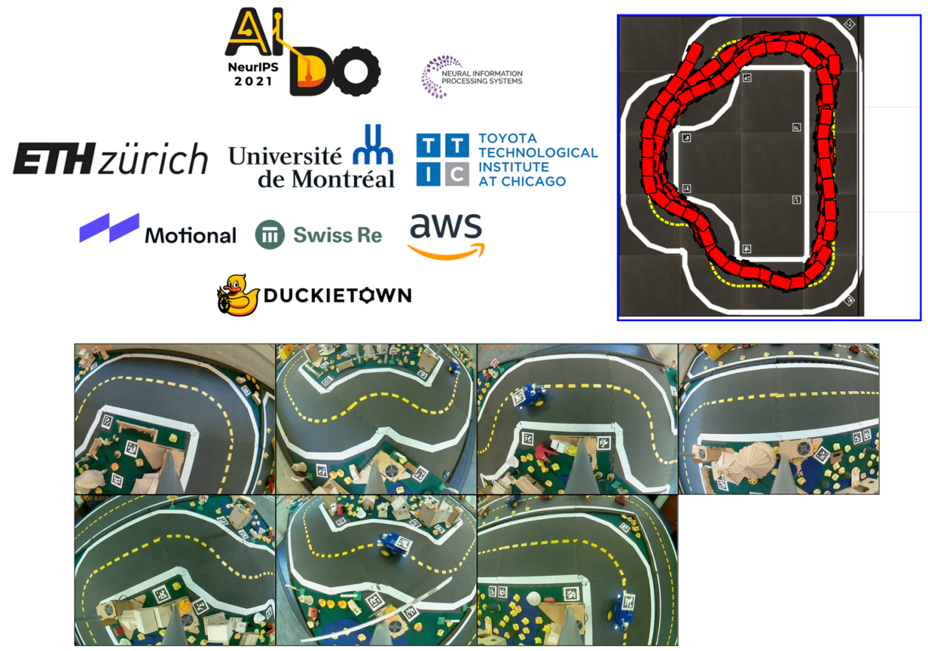
From 2018-2021 we ran several editions of the AI Driving Olympics (AI-DO): an international competition to benchmark the state of the art of embodied AI for safety-critical applications. It was a great experience – not only because it led to the development of the Challenges infrastructure, the Autolab infrastructure, and many agent baselines that catalyze further developments that are now available to the broader community, but even because it was the first time physical robots were brought the world’s leading scientific conference in Machine Learning (NeurIPS: the Neural Information Processing Systems conference – known as NIPS the first time AI-DO was launched).
All this infrastructure development and testing might have been instrumental in making R&D in autonomous mobile robotics more efficient. Practitioners in the field know-how doing R&D is particularly difficult because final outcomes are the result of the tuple (robot) x (environment) x (task) – so not standardizing everything other than the specific feature under development (i.e., not following the ceteris paribus principle) often leads to apples and pair comparisons, i.e., bad science, which hampers the overall progress of the field.
We are happy to see Duckietown recognized as a contributor to facilitating the making of good science in the field. We beleive that even better and more science will come in the next years, as the students being educated with the Duckietown system start their professional journeys in academia or the workforce.
We are excited to see what the future of robot autonomy will look like, and we will continue doing our best by providing tools, workflows, and comprehensive resources to facilitate the professional development of the next generations of scientists, engineers, and practicioners in the field!
To learn more about Duckietown teaching resources follow the link below.

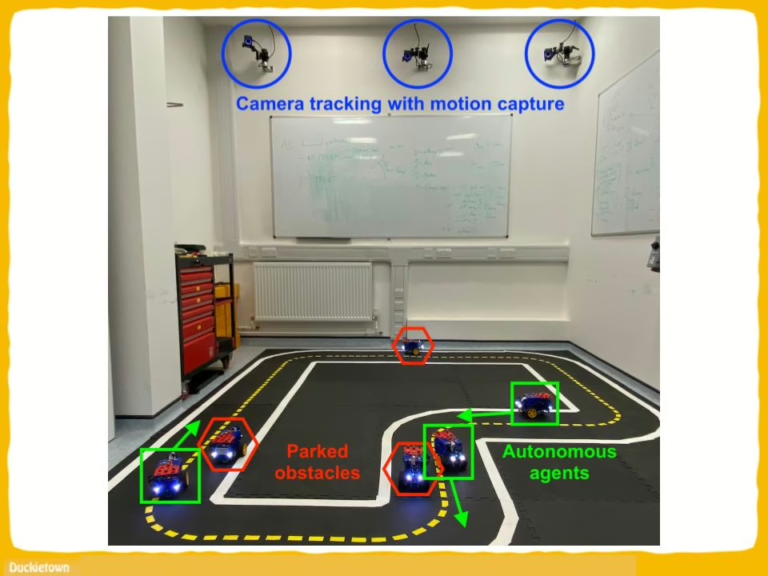
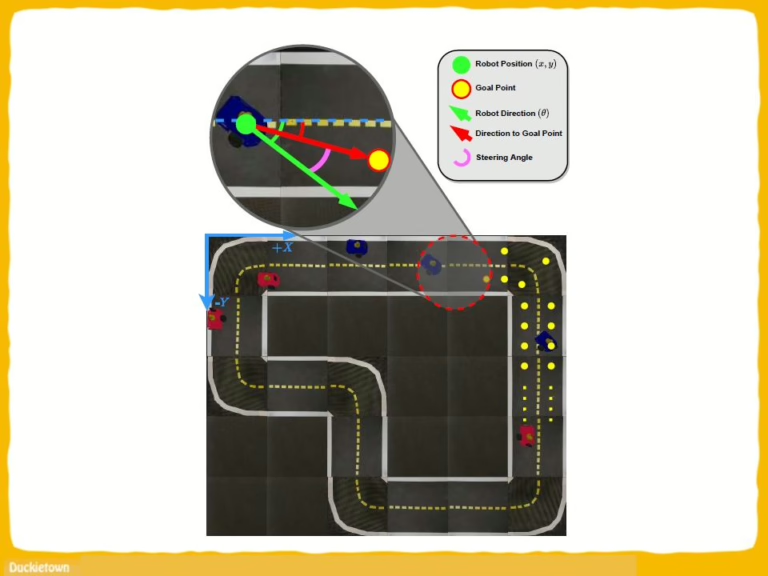


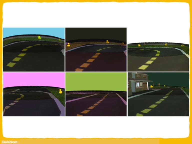
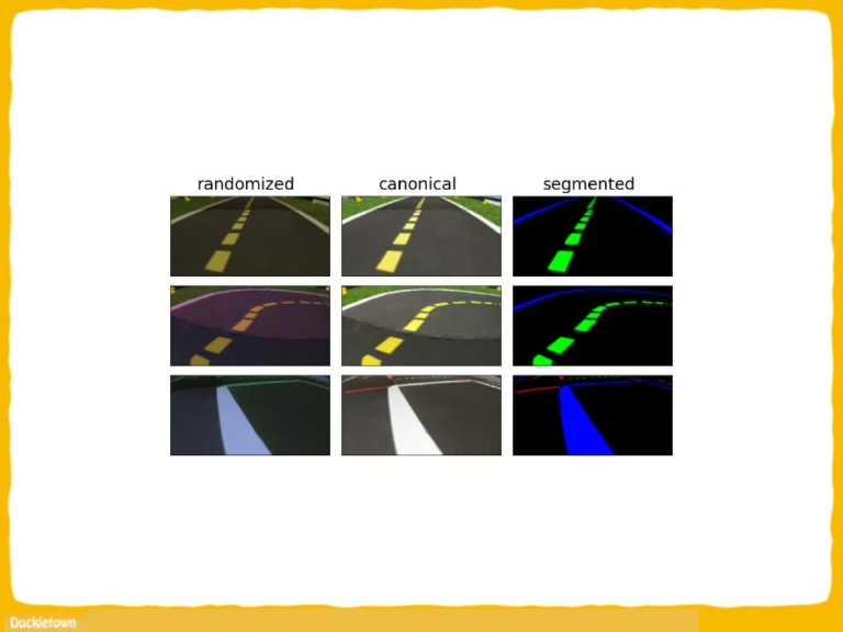
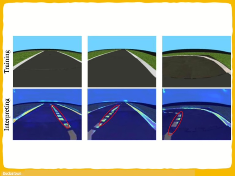
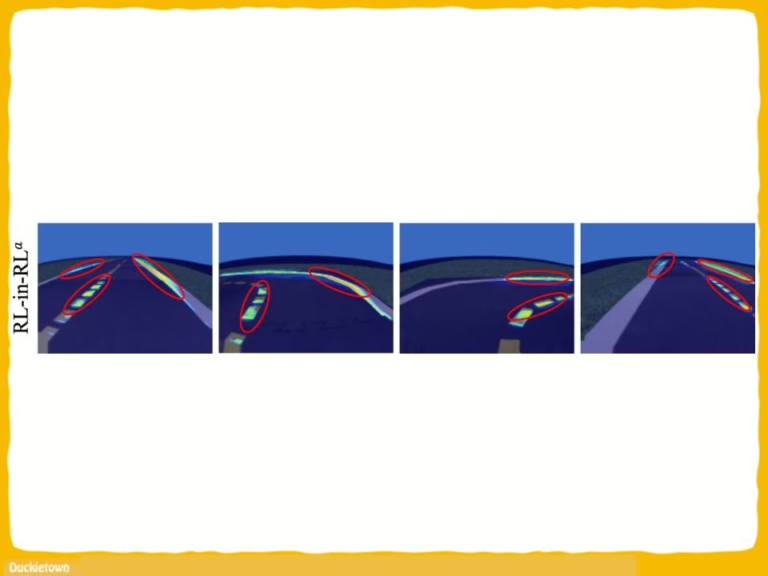
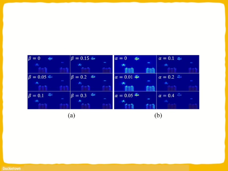
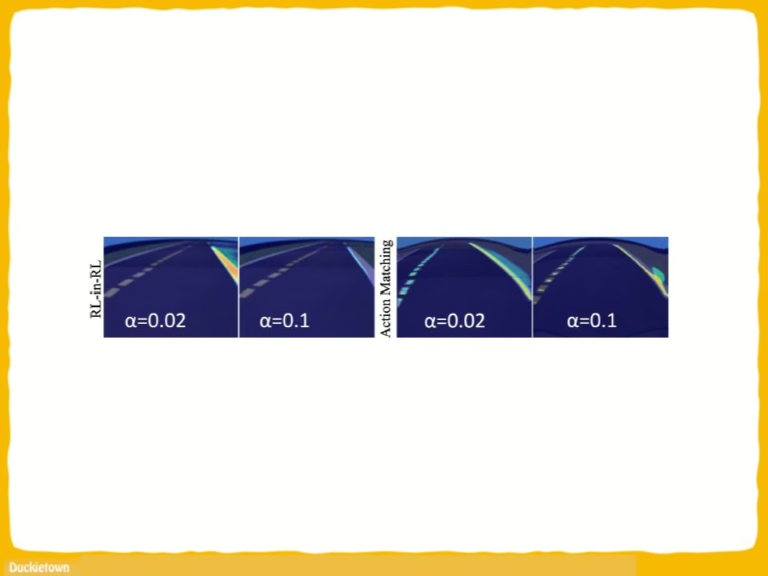
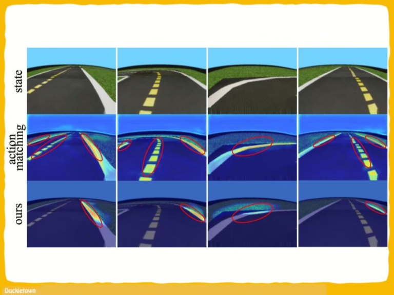
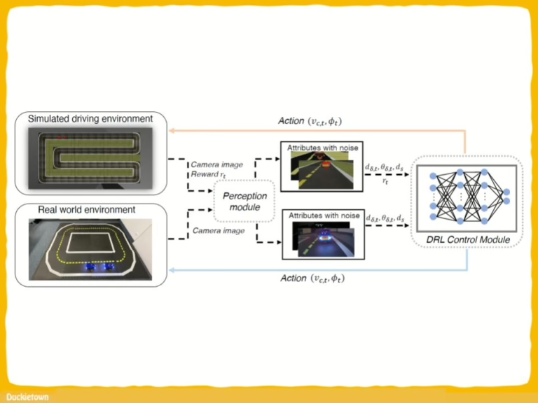
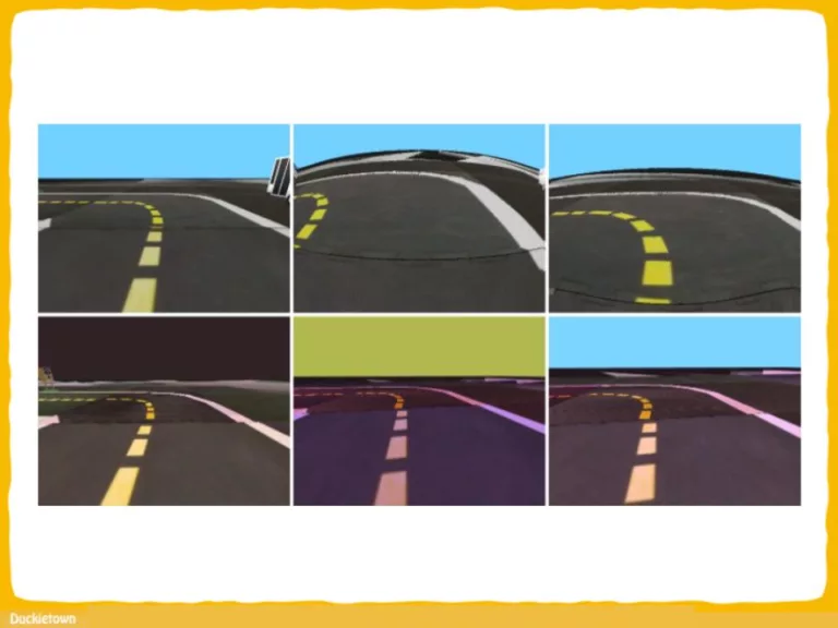
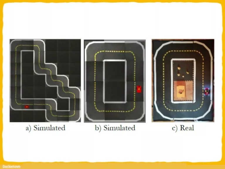
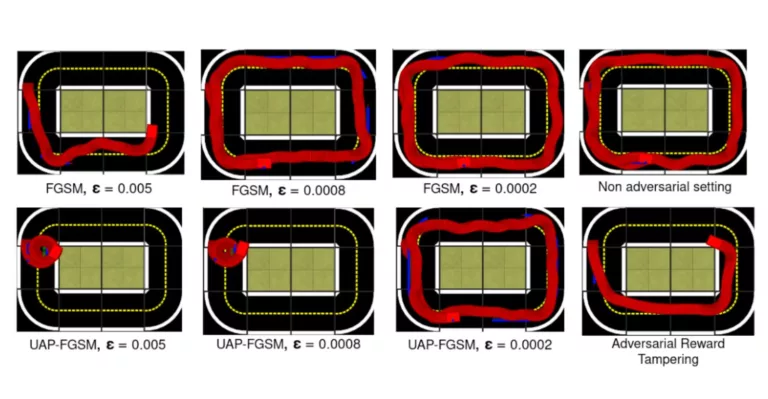
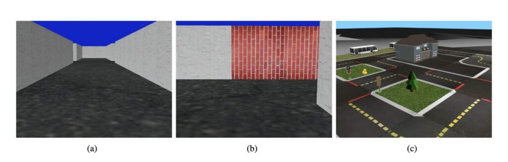
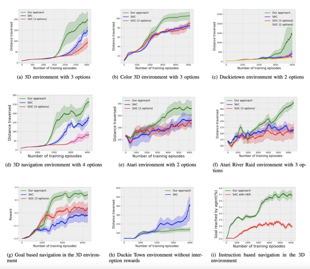
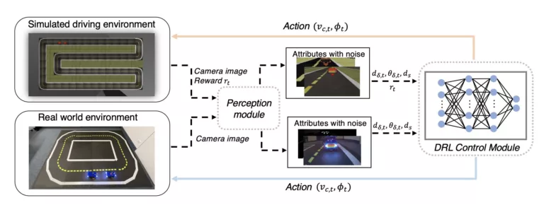
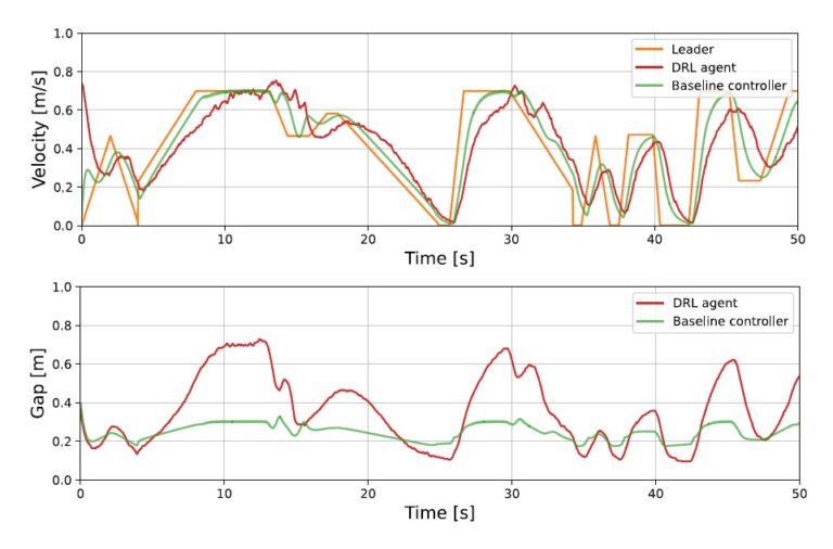
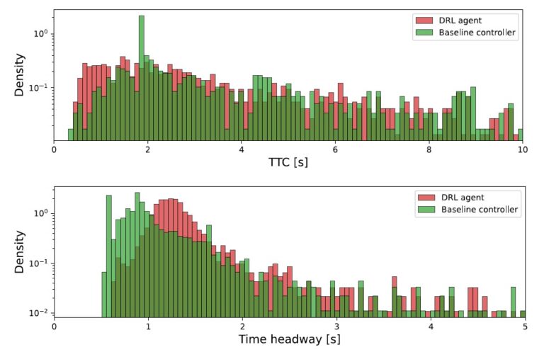
 Test track used for simulated reinforcement learning and baseline evaluations; b) and c) real and simulated test track used for the evaluation of the simulation-to-reality transfer - Duckietown")


 - Duckietown")